I wanted to test a fairly literal version of “more intelligence with less model”: if a small network can reuse the same computation, can it solve harder problems simply by thinking for longer?
The short answer is a qualified yes, at a much smaller scale than the phrase suggests. The reliable gains from extra recurrent compute only appeared after training across a range of reasoning depths. Where they did appear, additional recurrent steps carried accurate prediction a few dependency hops farther—single digits, not the tens of steps that “just let it think longer” implies. Past a sweet spot, more steps actively hurt. And I cannot yet tell whether those extra hops are the algorithm running or a shortcut my graph generator leaks.
Getting to that answer depends on being careful about what “reasoning depth” means, because the obvious way to measure it is badly misleading. I deal with that before any results, since it determines how every number below should be read.
The Setup
I used CLRS-style graph prediction tasks, but generated topology-controlled graphs so that problem size and dependency depth could be varied independently. That distinction matters: a graph can have more nodes without requiring a longer chain of dependent updates.
Four deliberately small models:
| Model | Parameters | What it tests |
|---|---|---|
| GRLS | 970,377 | My gated recurrent model with slots and deep supervision |
| GRU | 980,825 | A plain recurrent baseline |
| Small Transformer | 986,937 | A parameter-matched non-recurrent baseline |
| 31L Transformer reference | 4,255,737 | A larger, 31-layer Transformer matched on inference compute |
The 31-layer model is the honest baseline for anything involving inference cost, so it is the one I compare against throughout. Where I say “Transformer” without qualification below, I mean this one.
Tasks were Bellman–Ford, Dijkstra, BFS, and Prim’s minimum spanning tree, each trained with three seeds. Recurrent models are evaluated at an explicit unroll budget T, which I state wherever it matters.
The work ran in phases, and I use those labels below to say which experiment a number comes from:
| Phase | What it covers |
|---|---|
| 2 | The original four-task suite: 4 algorithms × 4 models × 3 seeds |
| 3 | Bellman–Ford across the four training conditions below |
| 4A | BFS replication at 32 nodes |
| 4B | BFS extended to 64 nodes, reaching measured dependency depth 47 |
| 4C | Re-scoring by exact dependency depth, restricted to the genuine-choice region |
| 4D | An audit of the generator’s own local structure |
Four training conditions, used from Phase 3 onward:
- Shallow: train only at requested depth 4, with recurrent unrolls sampled from 2–12.
- Depth mixture: train on requested depths 2, 4, 6, and 8, with unrolls still sampled independently.
- Coupled: the same depth mixture, but with the training unroll budget tied to each example’s measured dependency depth.
- Hint: the coupled condition plus intermediate algorithm-state supervision.
How I Measure Reasoning Depth
Three metrics are available, and the choice between them changes the answer by an order of magnitude.
Aggregate node accuracy at a requested depth is the obvious one, and it is the one that misleads. A graph requested at depth 48 does not contain only depth-48 nodes. Its deepest node sits at measured depth 47, but its mean node depth is about 19.8.
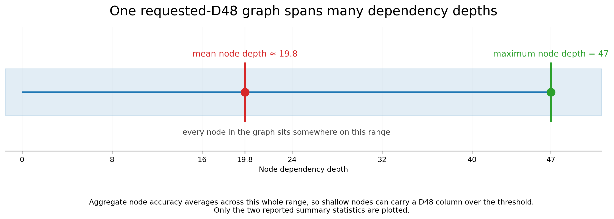
Averaging across that range lets easy shallow nodes carry an entire deep column. Scored this way in Phase 4B, the GRU cleared a floor-relative threshold all the way through D48 at every inference budget, including T=1. A one-step model does not perform 47-hop reasoning; the metric was reporting the shallow majority.
Whole-graph accuracy fails in the opposite direction. Requiring every node in a graph to be correct drives accuracy to effectively zero beyond D12 for every model, which is too coarse to locate where reasoning actually breaks.
Accuracy conditioned on each node’s exact dependency depth is much better, and it is my primary measure. For a headline number I report reach: the deepest contiguous exact dependency depth, starting from depth 2, that stays at or above a fixed accuracy threshold. The headline threshold is 0.80—an absolute bar, and a deliberately harsh one.
But exact-depth conditioning is still not sufficient on its own, because a generator can make deep nodes trivial. In the 64-node D48 generator, nodes at depths 18–47 have only one candidate parent: the pointer is structurally forced, so accuracy there measures the topology rather than the model. The Phase 4C depth-scaling analysis is therefore restricted to the genuine-choice region, exact depths 2–17, where every node has exactly two candidate parents.
Even that is not the whole story, for reasons the Phase 4D audit below makes clear.
The same pooling flattered the 32-node results, where it put every depth-mixture model at or past the D24 top of the evaluation grid.
I still quote requested-depth aggregates in the compute comparisons below, because the FLOPs-matched sweeps were run on that axis. Where I do, I label them as aggregates and I do not read them as reasoning depth.
Training Across Depths Is What Makes Depth Generalization Work
Under shallow training, all three architectures degrade quickly as Bellman–Ford dependency depth grows:
| Requested depth | Transformer | GRU | GRLS |
|---|---|---|---|
| 4 | 0.992 | 0.995 | 0.994 |
| 8 | 0.816 | 0.920 | 0.911 |
| 12 | 0.590 | 0.748 | 0.705 |
| 16 | 0.464 | 0.622 | 0.577 |
| 24 | 0.363 | 0.466 | 0.461 |
Recurrence helps here, but not indefinitely: at depth 24 the trivial baseline was 0.460, so neither recurrent result is meaningfully above chance.
Changing the training distribution changes this far more than changing the architecture. At requested depth 16:
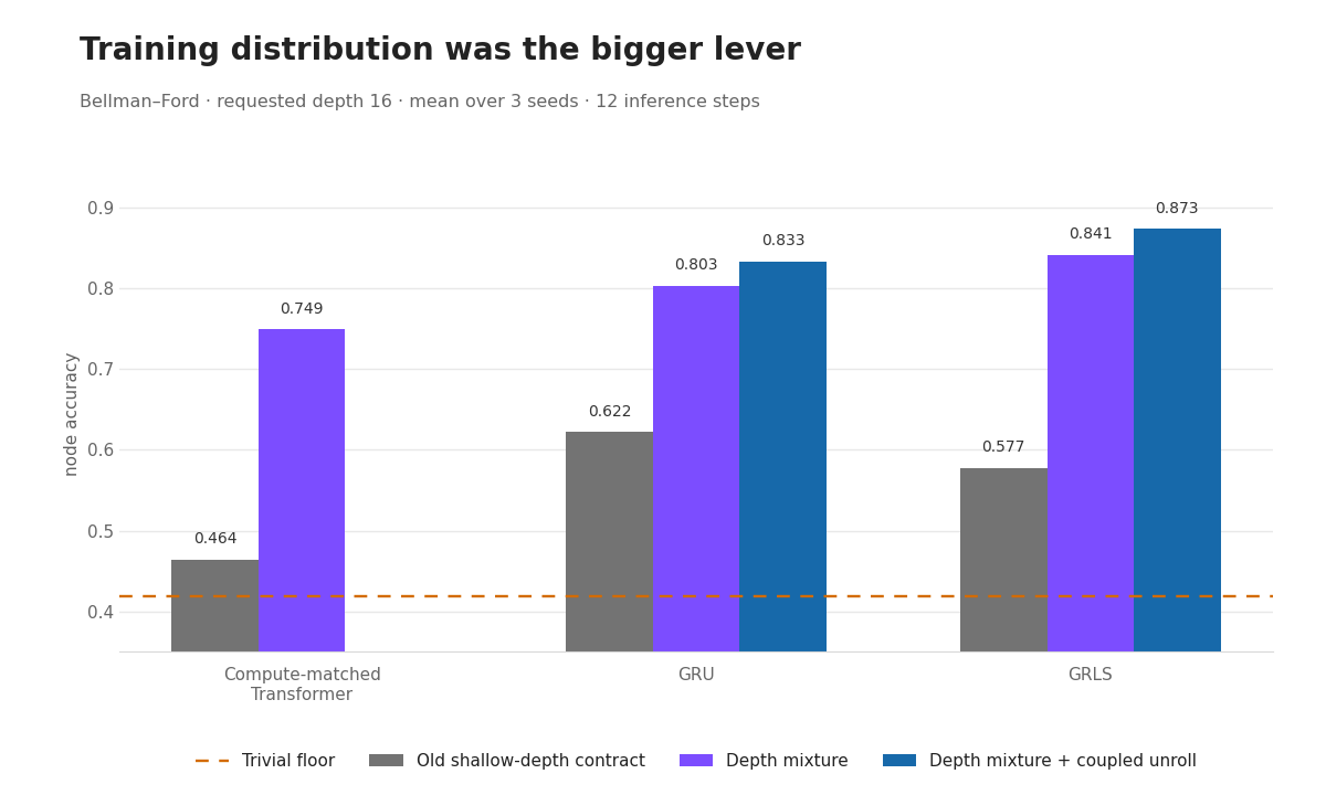
| Model | Shallow | Depth mixture | Coupled |
|---|---|---|---|
| Transformer | 0.464 | 0.749 | — |
| GRU | 0.622 | 0.803 | 0.833 |
| GRLS | 0.577 | 0.841 | 0.873 |
Depth-mixture training adds 0.285 for the Transformer, 0.181 for the GRU and 0.264 for GRLS. Coupling the budget to measured depth adds a further 0.030 and 0.032—real, but an order of magnitude smaller.
Phase 4A reproduces the same effect on BFS, a genuinely different algorithm, at 32 nodes:
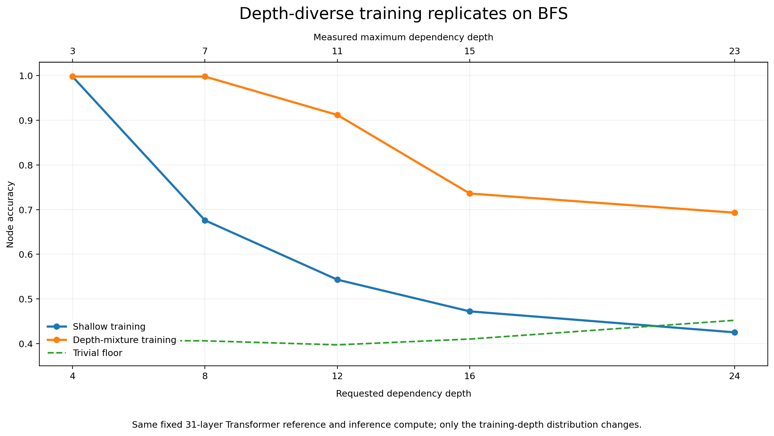
| Model | Training | D8 | D12 | D16 | D24 |
|---|---|---|---|---|---|
| Transformer | Shallow | 0.676 | 0.543 | 0.472 | 0.425 |
| Transformer | Depth mixture | 0.998 | 0.912 | 0.736 | 0.693 |
GRU (T=12) |
Shallow | 0.744 | 0.551 | 0.458 | 0.440 |
GRU (T=12) |
Depth mixture | 0.996 | 0.960 | 0.881 | 0.767 |
GRLS (T=12) |
Shallow | 0.783 | 0.616 | 0.524 | 0.495 |
GRLS (T=12) |
Depth mixture | 0.951 | 0.904 | 0.823 | 0.820 |
The Transformer row is the control that makes this convincing. Its inference is fixed—same 31 layers, same computation per example, under both training conditions. It cannot be spending more compute on harder examples, so the improvement has to come from the training distribution alone.
Training at one shallow depth teaches a finite-depth shortcut. Varying depth during training is what makes all three architectures learn something more general.
Recurrence Buys Accuracy Per Unit of Inference Compute
Training distribution determines whether a usable computation is learned at all. Recurrence is about how efficiently it runs.
In the Phase 4A compute sweep at 32 nodes on BFS, against a Transformer costing about 5.63 × 10^8 FLOPs per sample:
| Model | Relative FLOPs | D12 | D16 | D24 |
|---|---|---|---|---|
| Transformer / depth mixture | 1.00× | 0.916 | 0.740 | 0.694 |
GRU / depth mixture, T=8 |
0.85× | 0.980 | 0.930 | 0.768 |
GRLS / coupled, T=12 |
1.01× | 0.960 | 0.888 | 0.747 |
GRLS / depth mixture, T=8 |
0.69× | 0.935 | 0.849 | 0.768 |
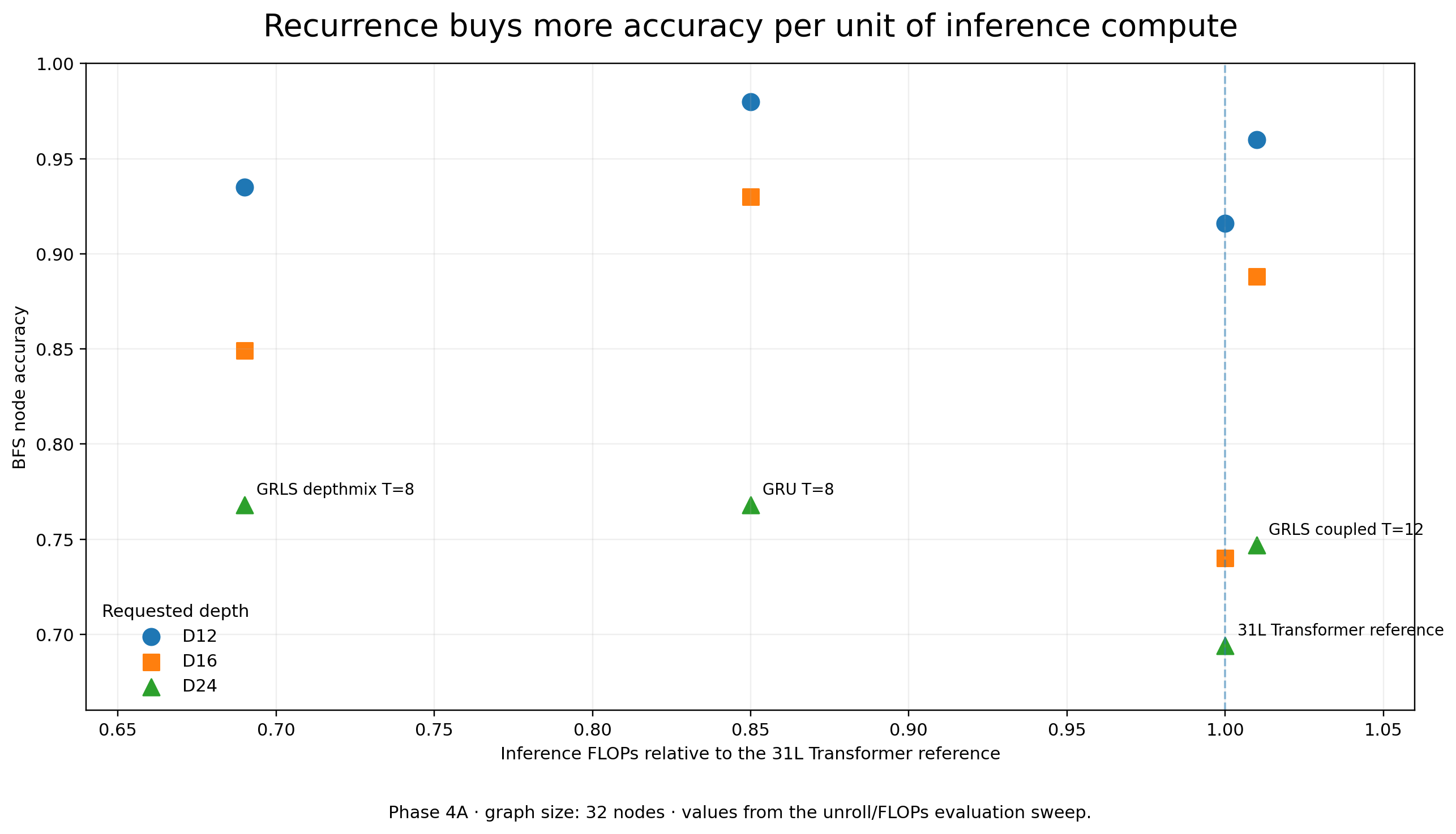
The Transformer values here (0.916 / 0.740 / 0.694) differ slightly from the table above (0.912 / 0.736 / 0.693) because they come from two evaluation slices: the depth table uses a fixed T=12 summary, this one uses the unroll/FLOPs sweep. I keep each slice’s own values rather than mixing them.
At 64 nodes in Phase 4B the original compute match no longer holds—attention scales more steeply with graph size—so this comparison uses measured cost rather than claiming the models are matched:
| Model | Relative FLOPs | D48 aggregate node accuracy |
|---|---|---|
| Transformer | 1.00× | 0.496 |
GRU, T=8 |
0.58× | 0.639 |
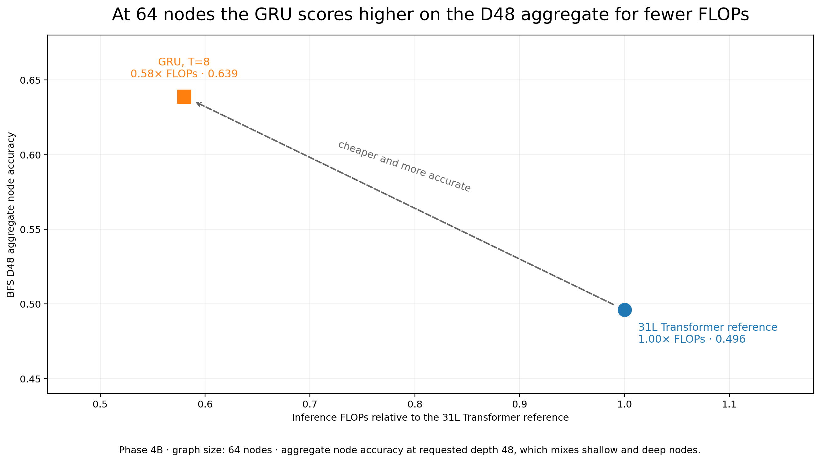
These are aggregate numbers, so read them as what they are: better partial prediction per FLOP. Neither model is executing a full 47-hop algorithm at D48. Recurrence gets more correct nodes per unit of compute, which is worth having and is not the same claim.
More Recurrent Compute Propagates Farther, Then Reverses
Scored by exact dependency depth, the deepest depth still reaching 0.80:
| Task | Graph size | Model / training | 0.80 reach, by seed |
|---|---|---|---|
| Bellman–Ford | 32 nodes | GRU / depth mixture | 4 / 5 / 2 |
| BFS | 32 nodes | GRU / depth mixture | 11 / 11 / 2 |
| BFS | 64 nodes | GRU / depth mixture, T=16 |
13 / 17c / 4 |
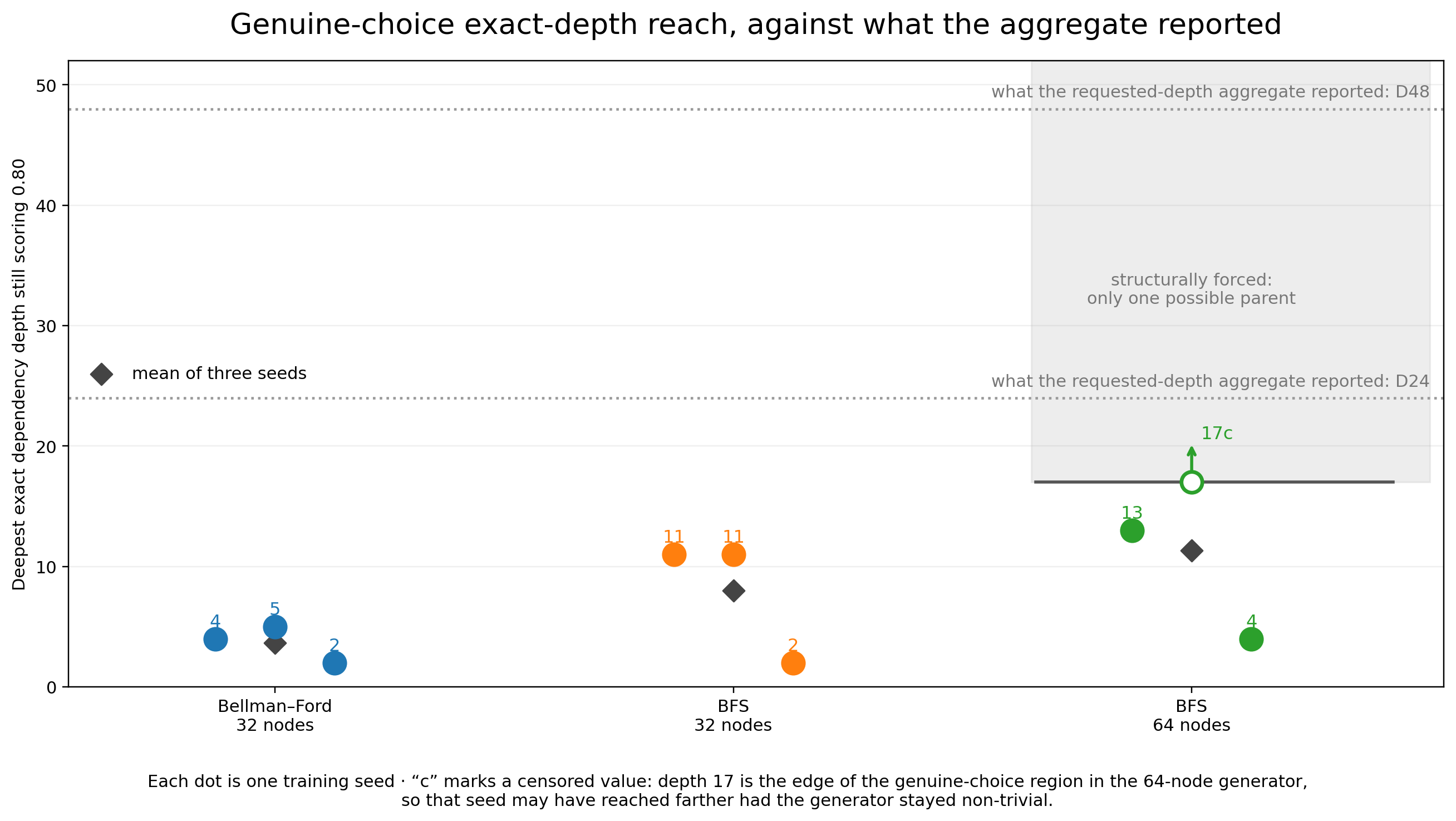
c means censored: depth 17 is the end of the genuine-choice region, so that seed may have reached farther if the generator had remained non-trivial.
Only the 64-node row comes from the Phase 4C restricted analysis, where the inference budget is T=16. The two 32-node rows are the stored Phase 3 and Phase 4A exact-depth back-check, scored under their original fixed evaluation budget; I do not quote an inference T for them here.
Read the upper end of that range with care. As The Generator Itself Contains a Structural Shortcut shows below, accuracy recovers from depth 14 up for reasons that have nothing to do with dependency reasoning, so a reach landing in that band is not evidence of reasoning to that depth.
These run from low single digits to the edge of the measurable genuine-choice region—far below what the requested-depth aggregate reports, and the honest scale of the effect.
Reach rises across those three settings in the means and in the stronger seeds, but they differ in task and graph size, not in recurrent budget—so that ordering is not by itself evidence about inference compute. It is also not uniform: the weakest seed sits at 2 in both 32-node settings before reaching 4 at 64 nodes.
The evidence about recurrent compute is within-setting: hold the 64-node BFS setting fixed and vary T alone.
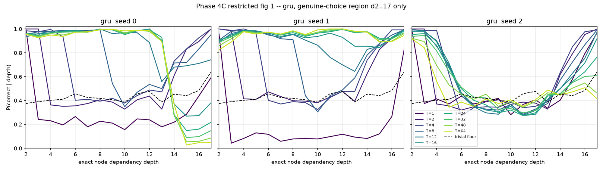
All three GRU seeds move outward as recurrent compute rises from T=1. Two move dramatically; the third only from depth 2 to about depth 4. In the two strong seeds the early progression is striking:
T=1 → 2, T=2 → 3, T=4 → 5, T=8 → 8, then roughly T=12–16 → 12–17.
I do not treat “one recurrent step buys one hop” as a law. One seed in three does not show it at all, and the generator audit below supplies an alternative explanation for part of the pattern.
And more is not monotonically better. At D48, performance peaked around the useful T≈8 region and fell by about 0.146 accuracy by T=64. GRLS was worse, losing roughly 0.39–0.41 aggregate accuracy between its best budget and T=64 at 32 nodes. Excessive recurrence reliably hurt, and how badly depends on the learned dynamics rather than on recurrence as such.
The Generator Itself Contains a Structural Shortcut
Phase 4D audits the generator rather than the models, and it matters more than any single result above.
The Phase 4B 64-node D48 layered generator spreads 63 non-source nodes over 47 layers. That does not divide evenly: early layers hold two nodes, later layers hold one. Node degree therefore changes near the far boundary—and that creates a purely local cue telling the model which direction points toward the source.
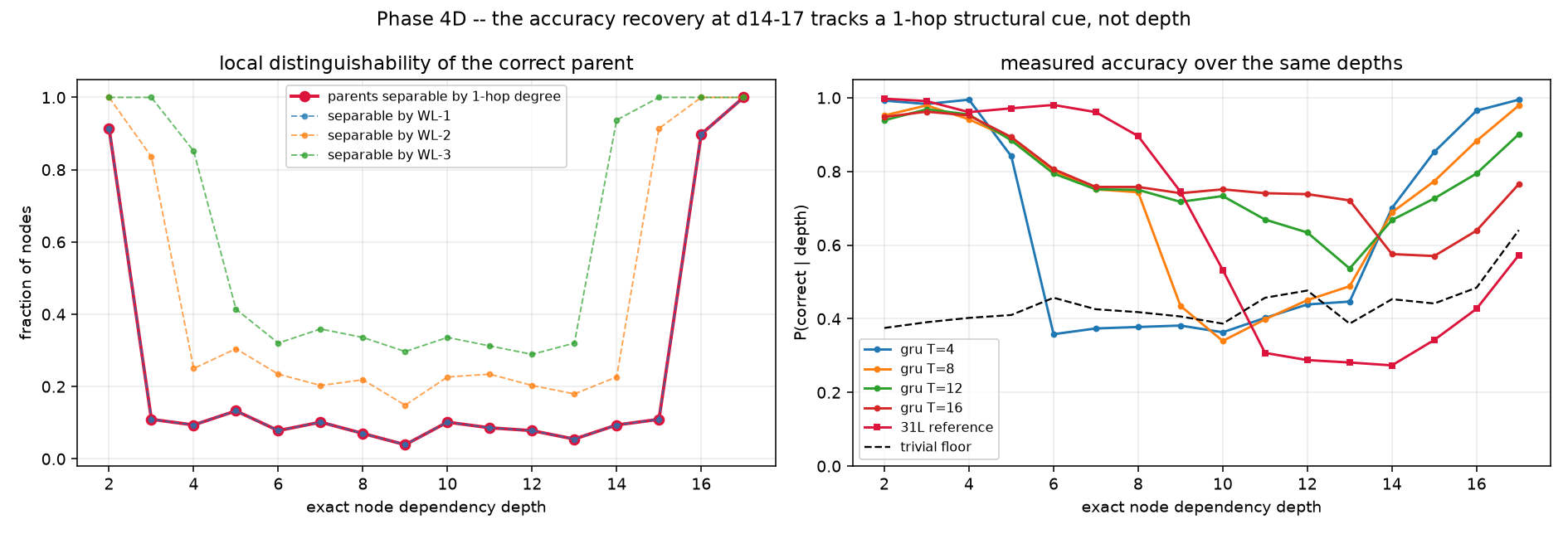
Every genuine-choice node at depths 2–17 still has exactly two candidate parents, so the late recovery is not caused by running out of choices. What changes is that the two candidates become locally distinguishable:
| Exact depth | Parent separability by degree | GRU T=4 |
GRU T=16 |
Transformer |
|---|---|---|---|---|
| 9 | 0.04 | 0.382 | 0.741 | 0.745 |
| 10 | 0.10 | 0.363 | 0.751 | 0.533 |
| 13 | 0.05 | 0.447 | 0.721 | 0.281 |
| 16 | 0.90 | 0.965 | 0.639 | 0.427 |
| 17 | 1.00 | 0.995 | 0.766 | 0.573 |
A purely local heuristic—keep the maximum-degree neighbours, then apply the normal tie-break—rises from roughly 0.36–0.43 in the interior to 0.637 / 0.957 / 1.000 at depths 15, 16 and 17. No dependency chain is followed anywhere in that procedure.
The decisive detail is that the fixed-depth Transformer recovers too, from 0.281 at depth 13 to 0.573 at depth 17. It cannot be executing more BFS steps—its computation is identical at every depth. A one-hop structural cue explains its recovery, and the same cue is available to the recurrent models.
Repeating the audit with Weisfeiler–Lehman neighbourhood signatures shows the boundary cue becoming visible farther inward as more hops of local structure are allowed, which is exactly what a model with more recurrent steps has access to.
So the evidence supports the weaker claim:
Additional recurrent steps propagate useful information farther through the graph.
It does not yet distinguish between two explanations:
- iterative execution of the intended BFS computation, and
- propagation of a structural boundary cue, or some other shortcut.
The least-confounded interior of this generator is roughly depths 5–13, where degree statistics are stationary and local separability stays low.
What Did Not Work
Intermediate supervision. One explanation for the depth limit was that endpoint supervision does not say enough about the intermediate computation. Supervising algorithm state along the way did not help:
| Model | Condition | Depth 16 | Depth 24 |
|---|---|---|---|
| GRU | Coupled | 0.833 | 0.631 |
| GRU | Hint | 0.762 | 0.613 |
| GRLS | Coupled | 0.873 | 0.631 |
| GRLS | Hint | 0.777 | 0.620 |
Hint models remained capable but were worse at depth 16 than endpoint-only coupled training.
Knowing the depth in advance. Coupling the unroll budget to measured dependency depth gave 0.030–0.032 over depth-mixture training on Bellman–Ford, and the BFS comparison had mixed signs. The depth distribution mattered; the oracle schedule barely did.
GRLS over a plain GRU. GRLS does not consistently beat the GRU on dependency depth. At depth 24 under coupled training they tied exactly (0.631 each), GRLS is substantially more vulnerable to excessive recurrence, and two of its three 64-node seeds diverged during training. The extra machinery has not earned itself yet.
A Note on Graph Size
Dependency depth and graph size are different axes, and recurrence behaves differently on each. Scaling BFS to 192 nodes:
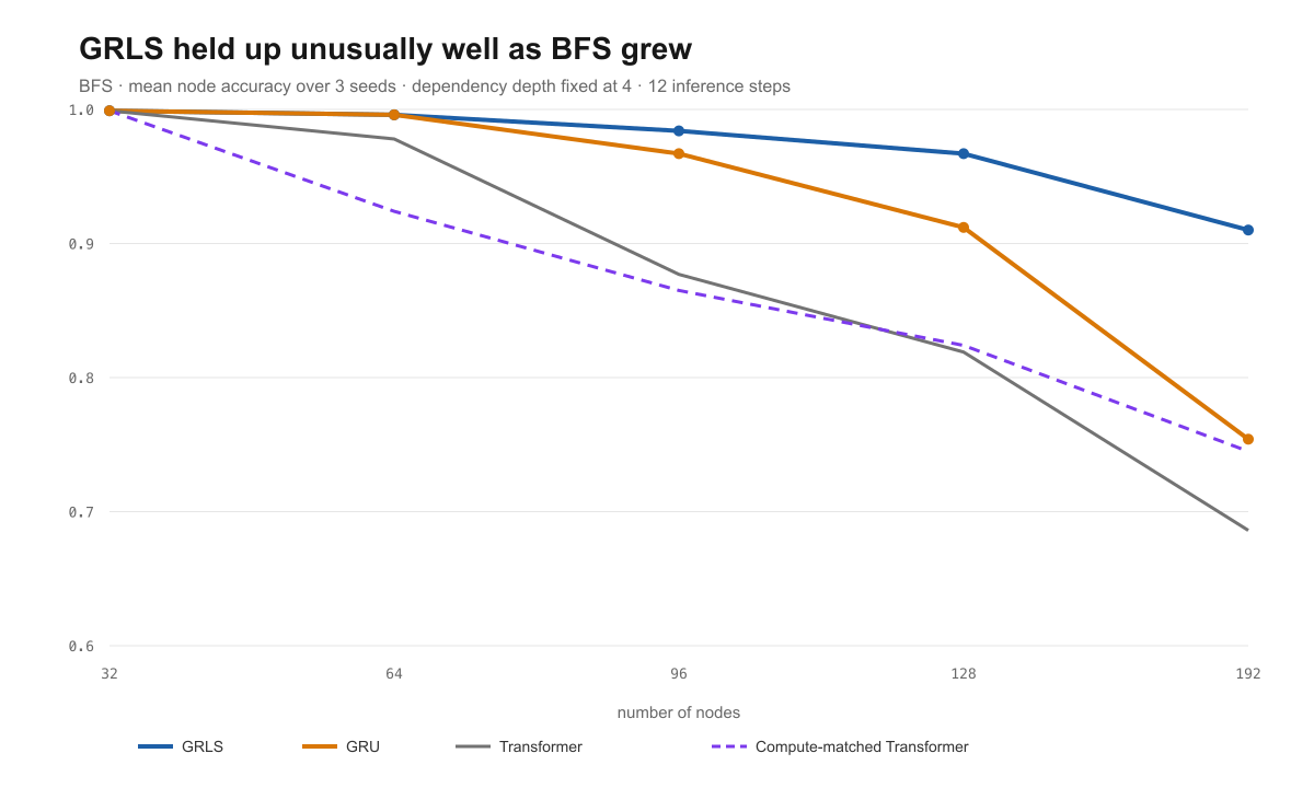
| Model | Node accuracy | Above trivial floor |
|---|---|---|
| GRLS | 0.910 | +0.482 |
| GRU | 0.754 | +0.326 |
| 31L Transformer reference | 0.745 | +0.316 |
| Small Transformer | 0.686 | +0.258 |
I would not generalize from this. BFS was the noisiest task in the suite: the three GRLS seeds scored 0.819, 0.940 and 0.972, while the 31L Transformer seeds scored 0.871, 0.849 and 0.513. On other tasks the ordering reverses—at 192 nodes on Bellman–Ford the 31L Transformer led with 0.965 against 0.941 for GRLS, and on MST it led 0.733 to 0.618. Size generalization is task-dependent, and three seeds cannot settle it.
Limitations
An evaluation bug affected the first Phase 2 pass. The recurrent-step budget could accidentally depend on an example’s trace length, so harder examples silently received different amounts of compute—contaminating exactly the comparison this experiment exists to make. I fixed the evaluator, added a regression test asserting the requested budget stays fixed, and re-scored all 48 original checkpoints without retraining. Every number in this article comes from the corrected evaluator.
The requested-depth frontier was never a reasoning-depth metric. It pooled shallow and deep nodes and saturated at the top of every evaluation grid, which is why it reported depths in the twenties and forties.
Dijkstra and Bellman–Ford are not independent. They used identical inputs and targets in the export, so they are one shortest-path result rather than two. The suite is three families—shortest path, BFS, MST—not four pieces of evidence.
The GRLS 64-node comparison is undertrained. Two of three seeds diverged; the checkpoint selector preserved earlier usable checkpoints, which leaves that comparison unsuitable for an architecture claim. I treat it as a stability diagnostic rather than as evidence for or against GRLS.
Three seeds is not many, and the seed spread within a single setting is large—2 to 11 at 32 nodes on BFS, 4 to 17c at 64 nodes. Point estimates in this article should be read with that spread in mind.
The generator leaks structural cues near its boundaries. The Phase 4D audit found that correct parents are locally separable at low depths and again from depth 14 up, so accuracy in those bands does not require following a dependency chain. This is the sharpest limitation in the study (the audit): it narrows the least-confounded range to roughly depths 5–13, where degree statistics are stationary, and it means any reach figure landing in the recovery band should not be read as reasoning depth.
The Phase 4B 64-node generator stops posing a real problem past depth 17. Beyond that every node has a single possible parent, so the deepest region of the graph cannot distinguish a model that reasons from one that follows the only available edge. This censors the strongest seed’s reach at 17c, and it means the true ceiling of depth scaling is still unmeasured—a generator that stays non-trivial deeper is the next thing I need.
The primary evaluation grid topped out at D24 for the 32-node experiments, so results there are bounded by the benchmark rather than by the models. Raising graph size to 64 nodes removed that ceiling, which is how the aggregate-metric problem became visible.
What I Conclude
Training across reasoning depths is the strongest and most robust effect. It improves extrapolation in every architecture, including a fixed-depth Transformer whose inference computation does not change at all. It reproduces on a second algorithm, and it survives the change of metric that cost the other results most of their magnitude.
Recurrence buys better partial accuracy per unit of inference compute. At 64 nodes the GRU reached 0.639 on the D48 aggregate against 0.496 for the Transformer, using about 0.58× the FLOPs.
Extra recurrent steps do carry accurate prediction farther, but the magnitude is highly seed-dependent and saturates quickly. At 64 nodes, the restricted 0.80 reach at T=16 is 13 / 17c / 4, versus 2 / 2 / 2 at T=1. Whether that extra reach is algorithmic execution or propagated structural cues is not something this generator can decide.
Measurement choice dominates the answer here. The same checkpoints can appear to clear a requested D48 aggregate while their genuine-choice exact-depth reach is only 4–17 nodes, depending on seed. That is the most transferable thing I found.
I started by asking whether a small model could learn an algorithm once and simply run it for longer when the problem became harder. I still cannot answer that, but I now know precisely what is blocking the answer:
Recurrence propagates computation farther with additional steps—but my current BFS generator cannot yet tell whether that computation is the algorithm or a structural shortcut.
One result is untouched by that ambiguity. The depth-training comparison holds training condition against training condition on identical graphs: both conditions see exactly the same structural cues, and the shallow-trained models are still far worse. Training across reasoning depths robustly improves extrapolation, and that stands regardless of how the cue question resolves.
Removing that ambiguity is a concrete piece of engineering, not a mystery: a generator with stationary layer occupancy, matched local degree statistics, constant parent-choice structure, and no depth-dependent local cue. If the rightward shift with T survives in that generator, the case for genuine iterative execution becomes much stronger. If it does not, I will have been measuring cue propagation the whole time.
I also want to know why the weakest seed stays stuck around depth 4 while its siblings track the recurrent budget almost hop for hop.
Phase 2: 48 checkpoints across the four-task suite. Phase 3: 30 further Bellman–Ford checkpoints across training conditions. Phase 4A: 24 BFS checkpoints at 32 nodes. Phase 4B: a nine-job 64-node BFS extension reaching measured dependency depth 47. Phase 4C: exact-depth measurement, restricted to the genuine-choice region. Phase 4D: a local-structure audit of the generator. Three seeds throughout unless noted. All depth claims use the corrected fixed-budget evaluator and exact-depth scoring, and the interpretation above incorporates the Phase 4D generator confound.